We regularly use tools like PostgreSQL, Pandas, and Jupyter Notebooks to analyze data here at Caktus. Recently, we were reviewing North Carolina traffic stop data for the NC CopWatch project and had the opportunity to use PostgreSQL's window functions, which are helpful when aggregating data.
To get an idea of why window functions are valuable, let's start with a simple example table:
SELECT
    stop_date
    , driver_race
    , driver_gender
FROM ncstops
ORDER BY stop_date DESC
LIMIT 10;
stop_date      | driver_race | driver_gender
---------------------+-------------+---------------
2022-10-31 22:28:00 | Black       | female
2022-10-31 20:04:00 | Hispanic    | male
2022-10-31 13:55:00 | Black       | male
2022-10-31 08:45:00 | Black       | male
2022-10-31 00:39:00 | Hispanic    | male
2022-10-30 20:00:00 | Black       | male
2022-10-30 19:53:00 | White       | male
2022-10-30 19:41:00 | Black       | female
2022-10-30 18:57:00 | Black       | female
2022-10-30 16:00:00 | Black       | female
(10 rows)
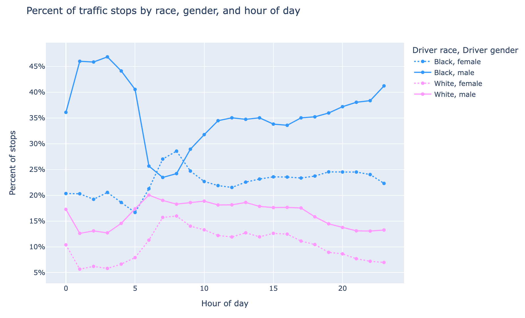
Using this data, say we want to get the percent of traffic stops by race, gender, and hour of day. For example, between 2-3a in the morning, what's the percentage breakdown of stopped drivers by race and gender.
First,
cast
the timestamp column to a time type to exclude the date portion. A
simple SELECT example can help illustrate:
traffic_stops_nc=# SELECT '2022-10-31 22:28:00'::time;
   time
----------
 22:28:00
(1 row)
Then use date_trunc to truncate the time to the hour so it can be grouped together:
traffic_stops_nc=# SELECT date_trunc('hour', '2022-10-31 22:28:00'::time);
 date_trunc
------------
 22:00:00
(1 row)
Now combine this method with a
count
aggregate function and GROUP BY clause:
SELECT
    date_trunc('hour', stop_date::time) AS hour_of_day
    , driver_race
    , driver_gender
    , count(*) AS stop_count
FROM ncstops
GROUP BY 1, 2, 3
ORDER BY date_trunc('hour', stop_date::time)
LIMIT 15;
hour_of_day |   driver_race   | driver_gender | count
-------------+-----------------+---------------+-------
00:00:00    | Asian           | female        |   300
00:00:00    | Asian           | male          |   636
00:00:00    | Black           | female        | 12065
00:00:00    | Black           | male          | 21407
00:00:00    | Hispanic        | female        |  1314
00:00:00    | Hispanic        | male          |  6464
00:00:00    | Native American | female        |    31
00:00:00    | Native American | male          |    73
00:00:00    | Other           | female        |   160
00:00:00    | Other           | male          |   461
00:00:00    | White           | female        |  6161
00:00:00    | White           | male          | 10246
01:00:00    | Asian           | female        |    42
01:00:00    | Asian           | male          |   126
01:00:00    | Black           | female        |  2231
(15 rows)
So how do we now calculate the percentage breakdown by hour? To start,
we want to divide the midnight count values above by the total
midnight stops, for example:
SELECT
    count(*) AS stop_count
FROM ncstops
WHERE date_trunc('hour', stop_date::time) = '00:00:00';
However, we want that for every hour. This is where we can use PostgreSQL's window functions:
SELECT
    date_trunc('hour', stop_date::time) AS hour_of_day
    , driver_race
    , driver_gender
    , count(*) AS stop_count
    , sum(count(*)) OVER (PARTITION BY date_trunc('hour', stop_date::time)) AS total_hour_stops
FROM ncstops
GROUP BY 1, 2, 3
ORDER BY date_trunc('hour', stop_date::time)
LIMIT 15;
hour_of_day |   driver_race   | driver_gender | count | total_hour_stops
-------------+-----------------+---------------+-------+------------------
00:00:00    | Asian           | female        |   300 |            59318
00:00:00    | Asian           | male          |   636 |            59318
00:00:00    | Black           | female        | 12065 |            59318
00:00:00    | Black           | male          | 21407 |            59318
00:00:00    | Hispanic        | female        |  1314 |            59318
00:00:00    | Hispanic        | male          |  6464 |            59318
00:00:00    | Native American | female        |    31 |            59318
00:00:00    | Native American | male          |    73 |            59318
00:00:00    | Other           | female        |   160 |            59318
00:00:00    | Other           | male          |   461 |            59318
00:00:00    | White           | female        |  6161 |            59318
00:00:00    | White           | male          | 10246 |            59318
01:00:00    | Asian           | female        |    42 |            10993
01:00:00    | Asian           | male          |   126 |            10993
01:00:00    | Black           | female        |  2231 |            10993
(15 rows)
Let's break this down. A window function performs a calculation across a set of table rows that are somehow related to the current row. We already have the count of stops, so we'll need to sum those counts across multiple rows:
sum(count(*)) OVER ()
However, we only want to sum rows within the same hour. The
PARTITION BY clause within OVER divides the rows into partitions
that share the same values of the PARTITION BY expressions. So here we
want to PARTITION BY the hour of the day:
sum(count(*)) OVER (PARTITION BY date_trunc('hour', stop_date::time)) AS total_hour_stops
That's it! Now the total_hour_stops contains the total of stops per
hour, regardless of how the SELECT statement groups the data using
GROUP BY. In our example, there are total 59,318 stops between 12:00a
and 1:00a in the morning.
Now that we have the data we need, we can use Pandas to load and prepare the data:
import pandas as pd

df = pd.read_sql(
    """
    SELECT
        date_trunc('hour', stop_date::time) AS hour_of_day
        , driver_race
        , driver_gender
        , count(*) AS stop_count
        , sum(count(*)) OVER (PARTITION BY date_trunc('hour', stop_date::time)) AS total_hour_stops
    FROM ncstops
    GROUP BY 1, 2, 3
    ORDER BY date_trunc('hour', stop_date::time)
    """,
    pg_engine,
)
df["hour_of_day"] = df["hour_of_day"].dt.components['hours']
df["percent_stops_for_race_gender"] = df.stop_count / df.total_hour_stops
And Plotly Express to visualize the data:
import plotly.express as px

mask = df["driver_race"].isin(["Black", "White"])
fig = px.line(
    df[mask],
    x="hour_of_day",
    y='percent_stops_for_race_gender',
    color="driver_race",
    title="Percent of traffic stops by race, gender, and hour of day",
    labels={
        'percent_stops_for_race_gender': 'Percent of stops',
        'hour_of_day': 'Hour of day',
        "driver_race": "Driver race",
        "driver_gender": "Driver gender"
    },
    color_discrete_sequence=(px.colors.diverging.Picnic[1], px.colors.diverging.Picnic[7]),
    height=600,
    markers=True,
    line_dash="driver_gender",
    line_dash_map={"male": "solid", "female": "dot"},
    line_group="driver_gender",
)
fig.layout.yaxis.tickformat = ',.0%'
fig.update_traces(textposition="bottom right")